Navigating the Ocean's Depths: A Whole New World of "Where Am I?"

For many decades now, whenever I read anything about the ocean or marine-themed articles, I encounter some variation of this sentence: "The ocean covers more than 70% of the Earth's surface, a vast and largely unexplored frontier teeming with mysteries and marvels waiting to be discovered." Humanity, for some reason, seems more interested in exploring space than in delving into our own planet's depths.

Embarking on an underwater journey with an Autonomous Underwater Vehicle (AUV) is like trying to navigate outer space, but with a twist—it's actually harder. Yes, you read that right. If space is the final frontier, then the depths of the ocean are the ultra-hardcore, expert-level dungeon. Why, you might ask. Well, for starters, space navigation has the luxury of a near-vacuum environment. Signals and communications travel freely, allowing satellites and spacecraft to communicate with the clarity of a morning bell. In the ocean's depths, it's a whole different game.

Over the next couple of months, in a series of articles, I will explain why the problem of underwater navigation remains unsolved in the 21st century. I will not focus on why humanity needs AUVs, because that could easily be a very different series of articles. But believe me, we need them badly.

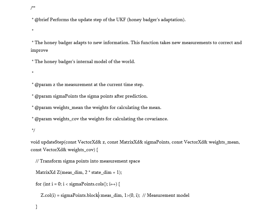
To begin, we consider the nuances of nonlinear dynamics and introduce the Unscented Kalman Filter (UKF). The UKF is a sophisticated tool that excels in scenarios where the traditional Kalman Filter will fail. From the elusive movements of wildlife to the precise navigation required by autonomous underwater vehicles, the UKF illuminates paths through the metaphorical fog with unmatched precision.

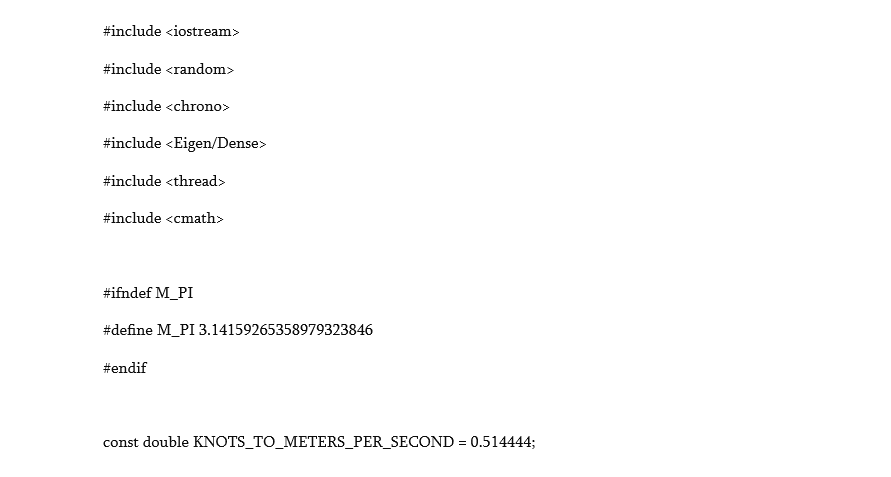
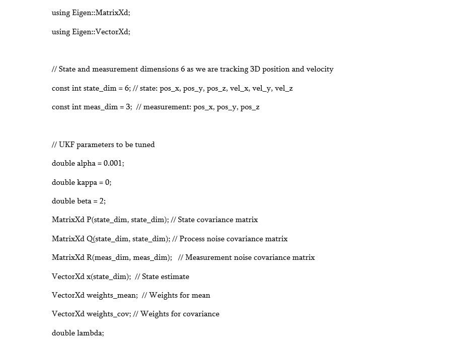
A unique aspect of this series is the practical implementation of these theoretical concepts in C++. Not only will we demystify the theoretical underpinnings of these filters, we will also roll up our sleeves and translate this knowledge into simple C++ code (I hope). This hands-on approach will bridge the gap between abstract mathematical concepts and their real-world applications, offering you a dual perspective on the challenges posed by marine navigation.

GPS Signals: "No Entry" Underwater

In space, GPS signals are the bread and butter of navigation. On Earth, you can hardly take a step without tripping over a GPS satellite signal. Let's face it, when navigating in space, you've got a clear line of sight to your cosmic road signs (thank you, vacuum of space). Underwater, navigating is like trying to complete a maze blindfolded, with one hand tied behind your back, while the maze is moving. Plus, it’s as though you're trying to follow a honey badger who's not keen on being followed. This honey badger (our dear AUV) doesn't walk; it glides, drifts, and sometimes dances to the tune of ocean currents. 

Underwater, GPS signals throw up a "No Entry" sign. They disintegrate into the aquatic equivalent of static before you get even a few meters below the surface. The signals may be able to travel for a couple of meters, but not always, and — even when they do — they don’t give exactly the right data flow. So, how do we navigate when our primary tool doesn't work? Enter the world of AUVs, where the mantra is "Expect the unexpected, and then some.”

GPS signals, which rely on high-frequency radio waves, encounter a significant barrier when they hit the water's surface. The electromagnetic nature of the signals means that they are absorbed and attenuated by water molecules, causing them to lose strength rapidly as they penetrate deeper. This rapid attenuation is due to the conductive properties of seawater, which disrupts the signal's ability to propagate. Consequently, even a couple of meters below the surface, the GPS signals become too weak and unstable to be detected or used for navigation. That almost completely removes the GPS navigation option for AUVs.

The Sensor Symphony (Or, The Slightly Out of Tune Orchestra)

As an engineer involved in the process of creating AUVs, I can tell you that the most efficient solution is to mimic human biology and equip AUVs with as many perceptual abilities as we can. That means we should engineer AUVs with the ability to see, hear, and have some kind of vestibular apparatus. It's a straightforward idea, but it’s very complicated to implement since we need to integrate these sensors into one cohesive perception system. Even if that can be done, this approach still faces serious challenges. Imagine yourself walking with a blindfold covering your eyes. After some time, your brain will adapt, and you’ll be able to more or less reach your destination — successfully walking from point A to point B. Now, imagine that you are doing this in a zero-gravity environment. Your body's sensors will start giving you a lot of calculation errors, making it nearly impossible for you to navigate.

The challenge of precise navigation arises not just with basic sensors but also with the most advanced and sophisticated mechanical or electronic sensors available; all are prone to errors in their output for various reasons. Consider, for instance, the IMU (Inertial Measurement Unit). This device measures and reports a body's specific force, angular rate, and (occasionally) the magnetic field surrounding the body. It does this using a combination of accelerometers, gyroscopes, and, in some cases, magnetometers. By measuring acceleration and angular rate, it provides crucial data that assists the vehicle in understanding its movement through the water. This information is vital for the vehicle's ability to navigate accurately without external reference points like GPS signals. However, like all sensors, IMUs are subject to inaccuracies and can actually contribute to the overall challenge of achieving precise navigation in AUVs.

To illustrate this with a practical example, consider the Movella MTi 600 Sensor Module, priced at approximately $1,604 USD. This module boasts a gyro bias stability of 10°/hr. Over a 15-day voyage, the maximum drift in angle could theoretically reach up to 3600 degrees. Although this is an unlikely and overly simplified scenario where the angular error accumulates in exactly the same direction, I could not resist using the simplification because of the huge figure that results. Such angular drift can lead to significant positional errors, particularly in long-duration missions like transatlantic crossings. Despite the MTi 600 providing high-quality data, the inherent limitations of IMU technology necessitate its use alongside other navigation systems to ensure accurate positioning over extended periods. In other words, even with quite an expensive sensor onboard, a mission starting in Lisbon and aimed for New York could, due to drifting error, inadvertently conclude in Havana. For me, that sounds quite acceptable since Havana is a really beautiful place. Since AUVs can’t really enjoy the beauties of Havana, and are not really into cigars, it is a huge problem for them. 

Ultimately, navigating an AUV is a bit like forming a band where each instrument plays its own tune — Inertial Measurement Units (IMUs) rock out on the vehicle's movements, Doppler Velocity Logs (DVLs) keep the rhythm with speed over the ground, and depth sensors hit the high notes with seafloor distances. Now imagine this band playing in a room filled with cotton — sounds get muffled, distorted, and sometimes lost. That's our sensor data. Valuable, but veiled in uncertainty, playing its heart out in the dense underwater fog.

Enter the Unscented Kalman Filter: The AUV's Compass in the Fog

In this whirlwind of noise and uncertainty, the Unscented Kalman Filter (UKF) steps in like an open fridge in the darkness of kitchen. It doesn't just slice through the darkness; it turns the darkness into its ally. The UKF grabs the chaos — the noise, the uncertainty, the hodgepodge of sensor data — and spins it into a story that makes sense. It forecasts where our elusive honey badger (the trusty AUV) will prance next, sharpening its predictions with each new morsel of noisy data.

Let's simplify this a bit. Imagine that, for some bizarre reason, you have a pet honey badger, and it's lost in the fog. Every so often, the honey badger yells for help (or perhaps it's just cursing the fog), and from those yells, you can roughly pinpoint its position, speed, and direction. Now imagine that, for an even stranger reason, you want your honey badger to find its way back to you. How would you guide it through the foggy abyss? That's where the Unscented Kalman Filter comes into play, acting as your virtual leash to bring your wayward honey badger safely back to you.

Before diving into the intricacies of the Unscented Kalman Filter, let's take a moment to explore the Kalman Filter itself — its origins, purpose, and a sprinkle of mathematical magic. Brace yourselves for a brief journey through formulas and quirky metaphors.

The Kalman Filter, introduced in the early 1960s by Rudolf E. Kalman, is the wise old sage of navigation and estimation theory. Born out of the need to guide spacecraft and missiles with precision, it became a cornerstone of aerospace engineering. Think of it as the GPS of its time, but instead of satellites, it relied on a clever blend of predictions and measurements to find its way.

At its core, the Kalman Filter operates using two fundamental steps: predict and update. Imagine that you're tracking our old friend, the elusive honey badger, through a dense forest — following the trail it left behind. This clever creature is known for its unpredictability, often doubling back on its path, or taking unexpected turns. The Kalman Filter comes to the rescue by helping you make an educated guess about where the honey badger's next paw print will be (prediction) and then adjusts that guess based on the actual tracks you discover (update). It's a continuous loop of guessing, checking, and refining, all wrapped up in a mathematical bow.

Now, why would we bring in the Unscented Kalman Filter? Well, just as our understanding of the world evolves, so do our tools. The Unscented Kalman Filter is like the Kalman Filter's adventurous grandchild, ready to tackle the nonlinear challenges that its predecessor found a bit too daunting. But before we unleash the power of the UKF, let's ensure that we're well-acquainted with the classic Kalman Filter, the foundation upon which our modern marvel stands. So, buckle up and prepare for a ride through the fascinating world of estimation theory, where every formula and metaphor bring us one step closer to mastering the unseen.

Now, it really is time for some formulas.

Background: Kalman Filter And It’s Unscented Descendant

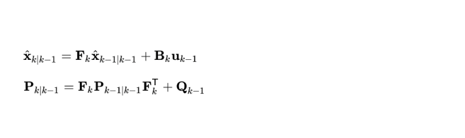
State Update Equation: This equation predicts the future state of the system based on the current state and the system's dynamics. If we consider our system state as x, and the system dynamics as F, the state update equation can be written as:

State Estimate (x̂k|k – 1): This represents our best guess of where the honey badger will be at the next moment, before we get any new information. It's like saying: based on how the honey badger has been moving so far, we think it will be at this particular spot next.

State Transition Matrix (Fk): This matrix describes how the honey badger's state (position and velocity) changes over time. It's like a set of rules that tells us how to update our estimate of the honey badger's position based on its current state.

Previous State Estimate (x̂k – 1|k – 1): This is our previous best guess of where the honey badger was. It's the starting point for making our new prediction.

Control Input Matrix (Bk) and Control Input (uk): In our honey badger scenario, these terms might not be directly applicable since the honey badger is moving of its own accord. In a controlled system, however, they would represent any external inputs or controls that influence the state of the system. For example, if we were remotely controlling a robotic honey badger, uk would be our control commands, and Bk would describe how those commands affect its movement.

Predicted Error Covariance (Pk∣k – 1): This represents our uncertainty about the prediction. Even with all of our calculations, we can't be 100% sure where the honey badger will go next. This term quantifies that uncertainty.

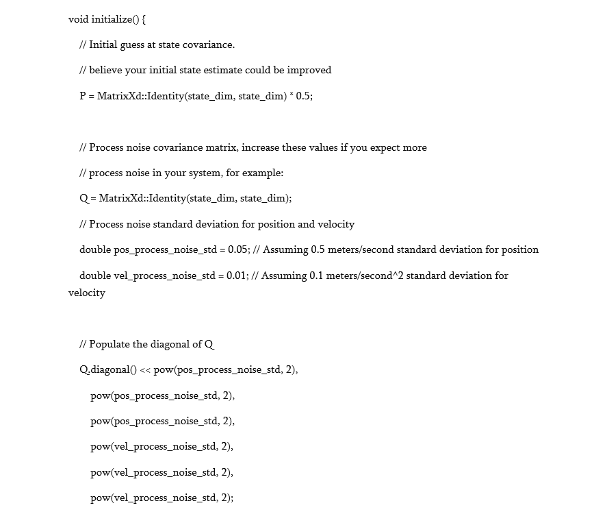
Process Noise Covariance (Qk): This accounts for any random, unpredictable factors that might affect the honey badger's movement. Maybe it suddenly decides to chase someone, or it encounters an obstacle that will regret meeting the honey badger. Qk represents the "noise" or variability in the honey badger's behaviour that our model doesn't capture.

After making our prediction about where the honey badger will be next, we receive new information — perhaps we hear a rustle in the bushes or spot some fresh tracks. This is where the update step comes into play, which is represented as:

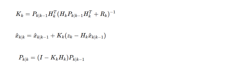
Kalman Gain (Kk): This is a crucial factor that determines how much we should trust the new information that we've received. It's like deciding how much weight to give to the latest clue about the honey badger's whereabouts. If the new information is reliable, we'll give it more weight. If it's uncertain, we'll rely more on our prediction.

Measurement (zk): This represents the new information that we've just received about the honey badger's position. It's the equivalent of hearing a rustle in the bushes and having a rough idea of where it came from.

Measurement Matrix (Hk): This matrix connects the honey badger's actual position to what we can measure. It helps us translate the raw sensor data (like the sound of the rustle) into an estimate of the honey badger's location.

Updated State Estimate (x̂k∣k = x̂k∣k – 1+Kk(zk−Hkx̂k∣k – 1)): This essentially combines the predicted state of our system (the location of our dear honey badger) with new observational data to produce a more accurate estimate of the state.

x̂k∣k: This is our revised best guess of where the honey badger is, considering both our prediction and the new information that we’ve received. It's like saying, "Based on what we thought before and what we've just heard, we now think the honey badger is here."

Updated Error Covariance (Pk∣k): This represents our updated uncertainty about the honey badger's position. Even with the new information, there's still some uncertainty, and this term quantifies it.

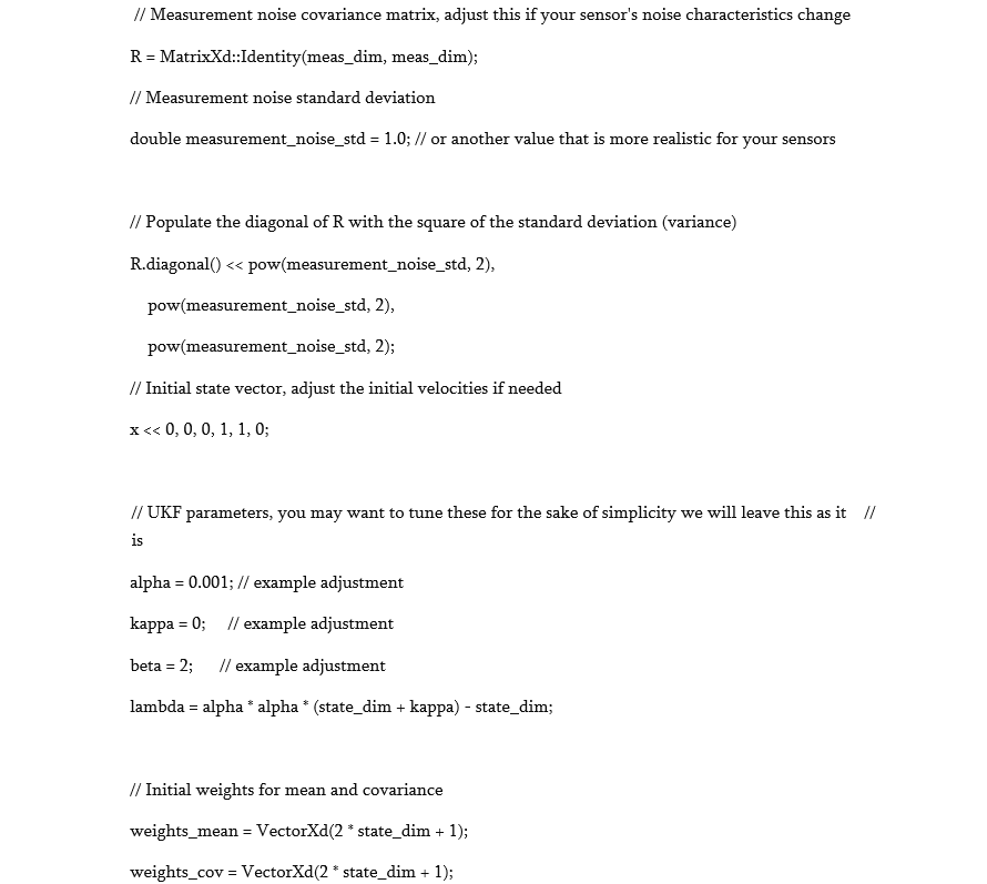
Measurement Noise Covariance (Rk): This accounts for the uncertainty in our measurements. For example, the rustle in the bushes might not be very clear, or there could be other animals moving nearby that confuse our sensors.

So, in the update step, we refine our prediction about the honey badger's position based on new information, adjusting our estimate to get closer to its actual location. It's like piecing together a puzzle. Each new clue helps us get a clearer picture of where our elusive friend is hiding in the forest.

Updated Tool: Unscented Kalman Filter

The Unscented Kalman Filter (UKF) is an extension of the classic Kalman Filter that is designed to handle nonlinearities in the system and measurement models. Let's continue our honey badger tracking expedition to see how the UKF improves our navigation through the non-linear forest terrain.

Imagine that our honey badger has eaten some fermented fruit, and its movement has become erratic and unpredictable. This represents a non-linear problem that the classic Kalman Filter might (and will) struggle with. The UKF addresses this by deploying a set of carefully chosen sample points, known as sigma points, to capture the mean and covariance of the honey badger's position accurately.

The following steps explain how the UKF works, continuing our honey badger metaphor:

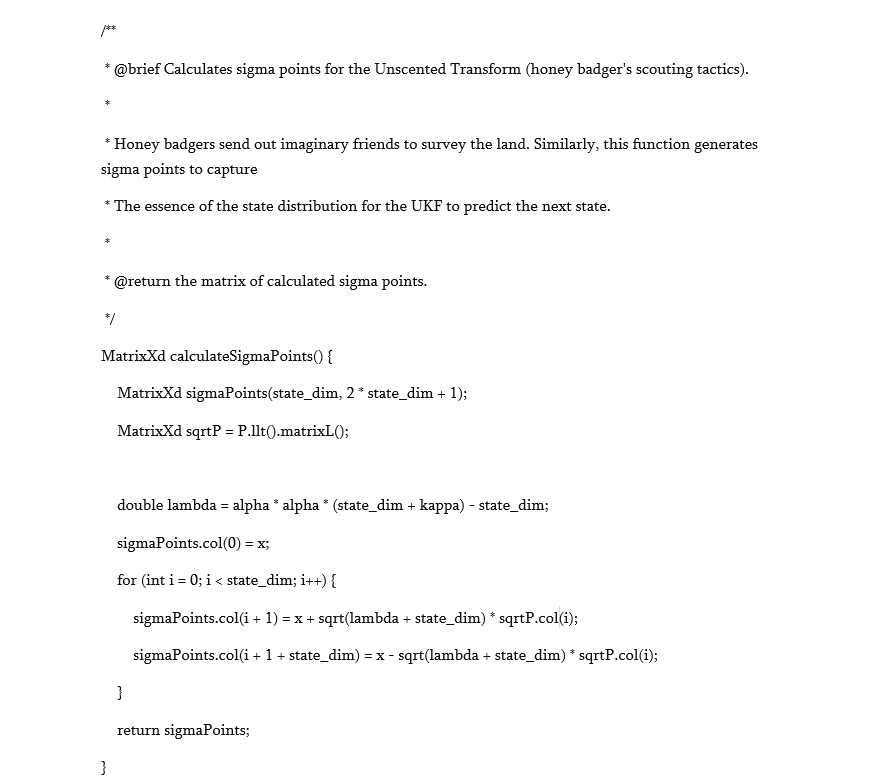
1. Sigma Points Selection: In the UKF, sigma points are selected from the probability distribution associated with the current state estimate These points are like a team of scouts, each taking a different path to predict where the honey badger might go next, considering its current state and the uncertainty in its movement.
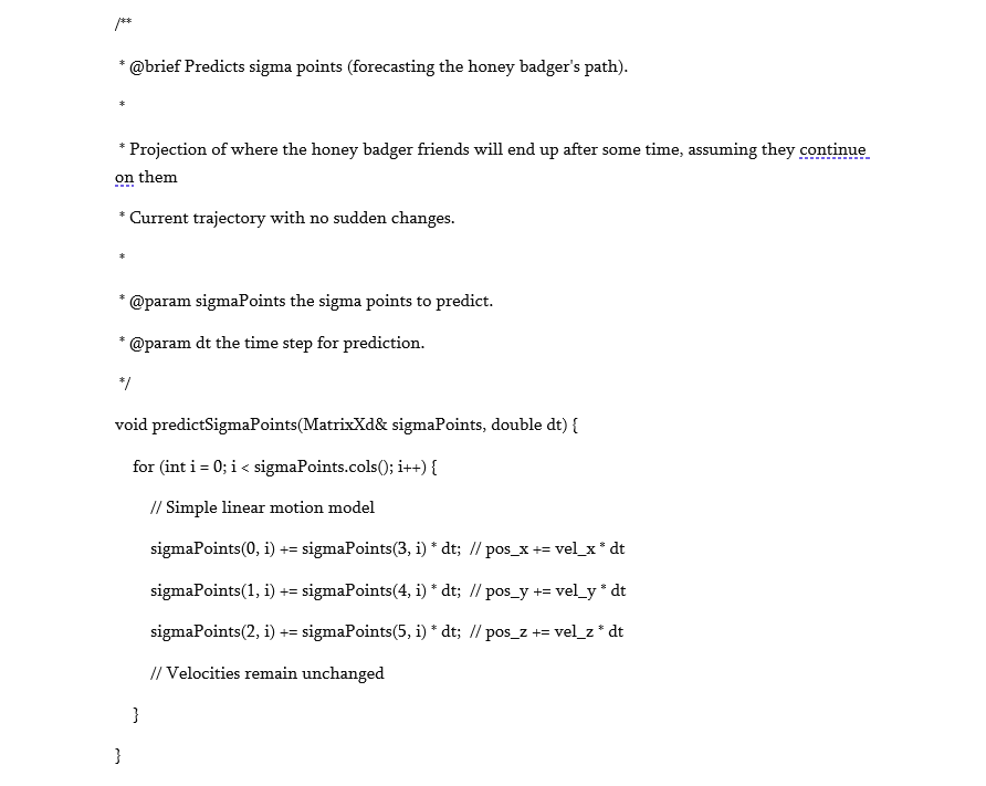
2. Transformation of Sigma Points: Each sigma point is then passed through the non-linear system model, this is akin to simulating how the honey badger might move through the forest. This step accounts for the possibility of the honey badger stumbling upon those fermented fruits and taking an unexpected leap.
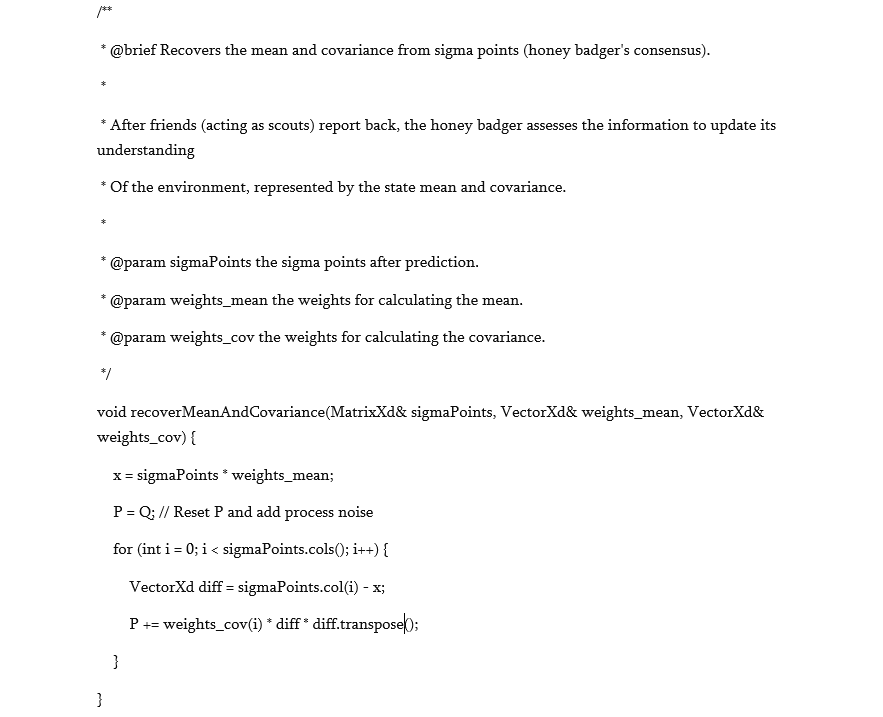
3. Prediction Step: After being passed through the system model, the transformed sigma points are then recombined to form a new mean and covariance estimate for the honey badger's position and velocity. This gives us a predicted state that includes possible non-linear paths that the honey badger might have taken.
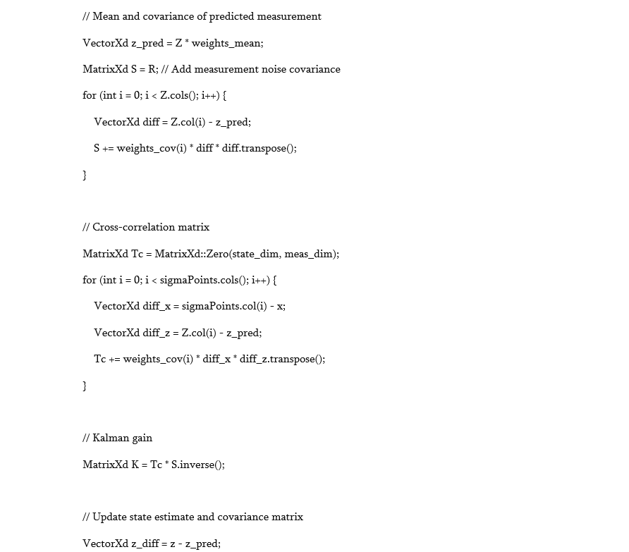
4. Incorporate Measurement: When new sensory information comes in — say, a snapped twig suggesting the honey badger's latest position — we use all of our sigma points to predict what we would have measured for each point. This prediction considers the non-linearity in how we measure the honey badger's position (like echoes distorting the sound in the forest).
5. Update Step: Finally, we combine our predicted measurements with the actual measurement to refine our state estimate. If the new data fits well with our predictions, we gain confidence in our estimate. If not, we adjust our sigma points to better match the reality, honing in on the honey badger's actual trail.

Through this process, the UKF maintains the essence of the Kalman Filter — predicting and updating — but with a powerful twist to handle the non-linear escapades of our honey badger. It's as if we've given our tracking team night-vision goggles, allowing them to see the twists and turns of the path more clearly, even when the journey takes unexpected turns.

Capturing Our Digital Honey Badger

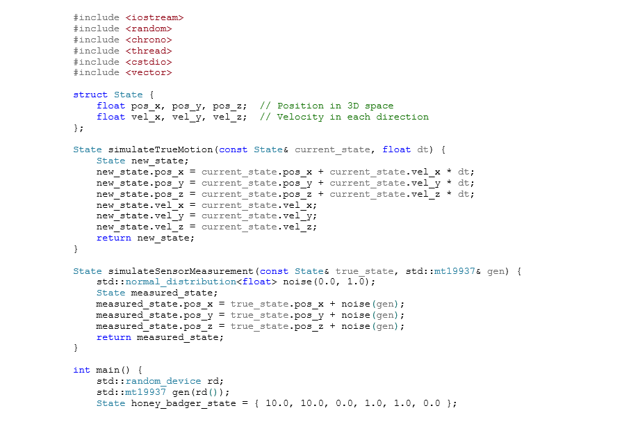
Before we dive into the realm of Kalman Filters, let's capture our metaphorical honey badger and equip it with an IMU sensor. I do not recommend doing this in real-life. But for now, imagine gently subduing our peaceful creature and fitting it with technology that will reveal all the secrets of its movement. Now, with our honey badger prepped, we're set to translate theory into practice, steering clear of ROS and other simulators. We're keeping it real with the hardcore C++.

Here's How We Tackle the Challenge

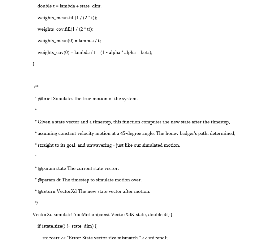
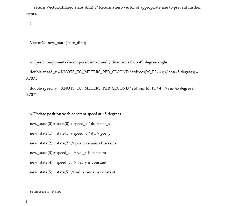
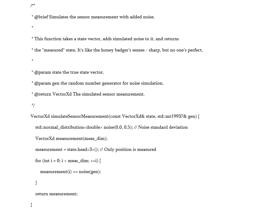
1. Simulate the IMU Sensor: We'll craft a function to mimic the output of an IMU sensor. This function will generate simulated readings of accelerations and angular velocities, peppered with a bit of 'noise' for realism. It’s about making our data as lifelike as possible without an actual frolicking honey badger.
2. Establish a Data Structure: A robust data structure is crucial to store our simulated IMU readings. This includes acceleration on three axes (yes, our honey badger can jump!), angular velocity, and possibly a timestamp to chronicle the exact moment that each piece of data was generated.
3. Implement the Prediction Step: With our faux sensor data in hand, we'll develop the prediction step of our Kalman Filter. This involves constructing the state transition matrix and control input matrix. Using these matrices, we’ll forecast the next state of our system based on our simulated data.
4. Integrate the Update Step: Once we have a predicted state, it’s time for corrections. We'll implement the update step, where our predicted state is adjusted according to the simulated measurements. The Kalman Gain comes into play here, fine-tuning our balance between prediction accuracy and the trustworthiness of our measurements.
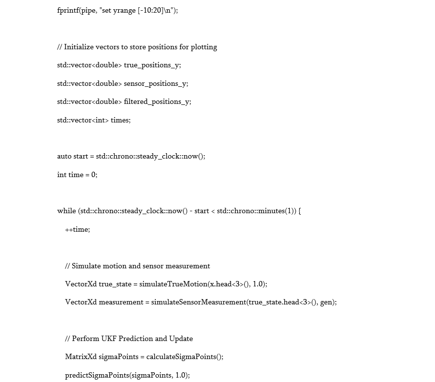
5. Track Three Trajectories: As we venture through this digital thicket, we’ll keep our eyes on three distinct paths: the real trajectory as it would occur without any sensor errors; the trajectory as perceived through the noisy lenses of our sensors; and the trajectory refined by the Kalman Filter.

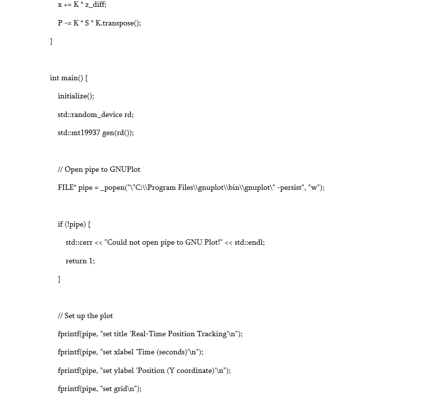
Ready for some hands-on action? We’ll start by simulating our IMU sensor data, breathing digital life into our theoretical honey badger. Follow along as we decode the movement of our elusive digital creature, exploring the intricacies of simulated reality versus sensor-imposed fiction and refined truth.

I try to keep things as simple as possible since we are only demonstrating the beauty of Kalman filtering, not building a production nav system for the AUV. 

Moving the Honey Badger

First let’s make it very simple.

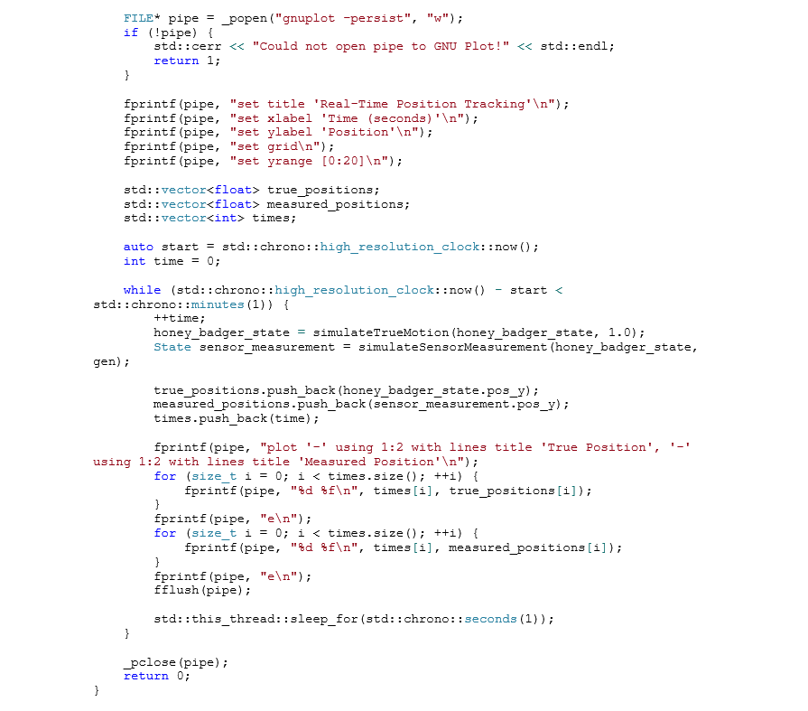
Ok, that will give us something like the clear linear movement shown below.

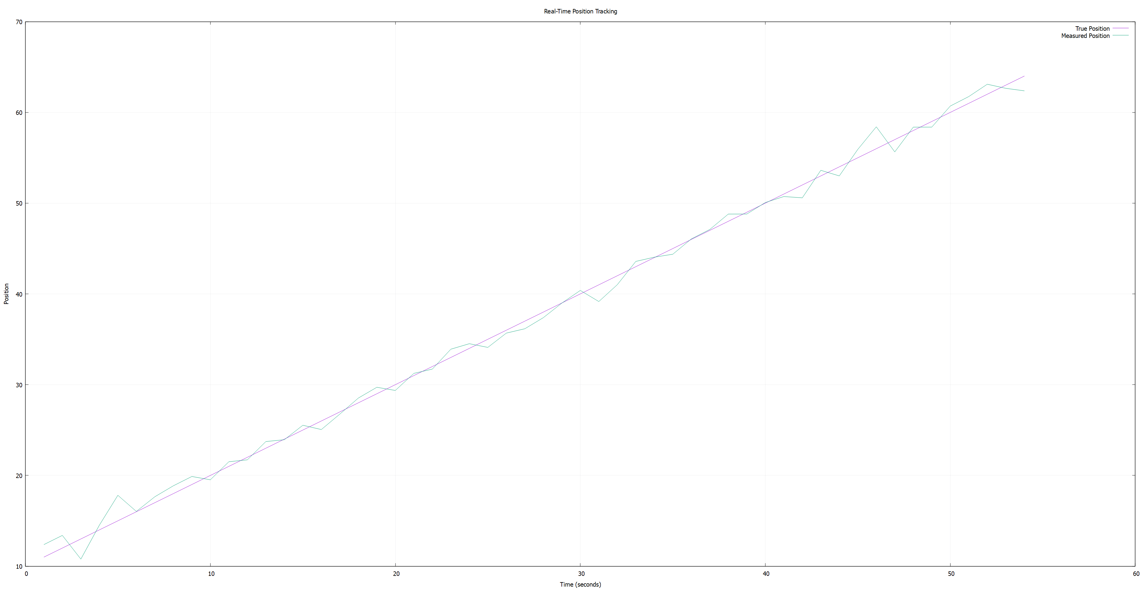
As we can see, the sensors give us data that is quite messy because of noise. In real life, we are going to see quite the same picture (or even worse, believe me). And, for our AUV, it is going to be difficult to proceed with nav decisions since those decisions will be based on very messy data.

Now, to implement Kalman Filtering, we need to use matrix operations and transformations as we would do in real life. So, the code will slightly (not significantly) change.

Making the honey badger smarter

If you have any intention of actually running this code, you should get Eigen and install GNU Plot to see the beautiful graph.

And here is what we get:

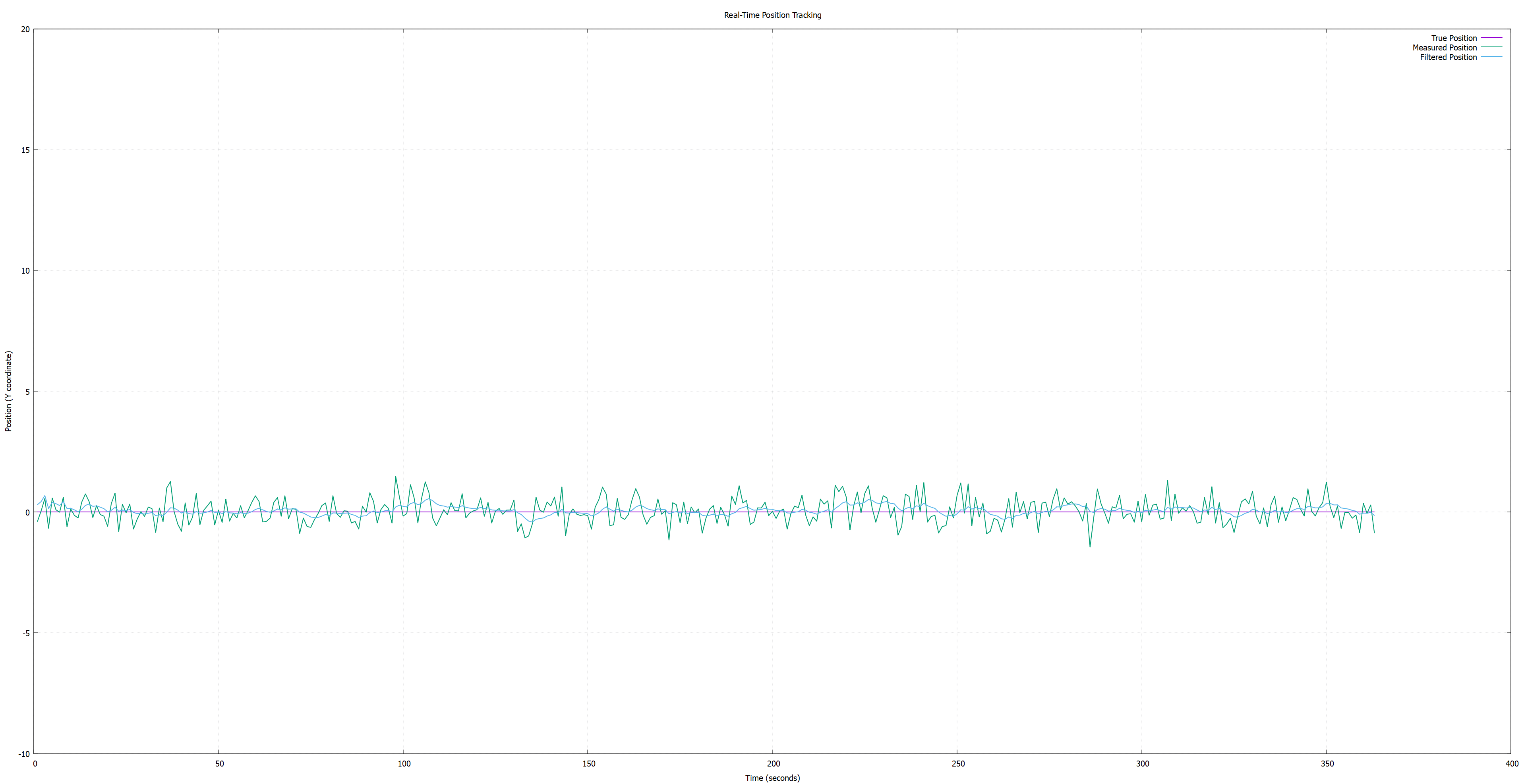
As shown above, the Unscented Kalman Filter (UKF) demonstrated substantial enhancement in the accuracy of positional estimates. The processed data, depicted in the filtered trajectory, exhibits significant improvement in both smoothness and in proximity to the actual path of the vehicle, underscoring the effectiveness of the UKF in addressing non-linearities inherent in dynamic systems.

Now is a good time for some real examples.

Let me introduce you to Typhoon AUV.

This is the mission course:

During a real-world deployment, critical navigational sensors were intentionally deactivated to emulate conditions akin to subaquatic travel, leaving only the Inertial Measurement Unit (IMU) and various filters operational. This scenario effectively mirrors the limitations faced by AUVs during submerged travel.

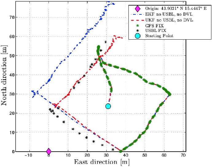
The empirical data collected from this mission starkly illustrates the limitations of conventional Kalman Filters, depicted by the blue dotted line, which could not provide a viable solution for the AUV’s navigation. The deployment of GPS was constrained to surface-level operation; upon submergence, its utility was rendered null. The implementation of the UKF, however, yielded a trajectory alignment nearly indistinguishable from that which would be obtained via GPS, highlighting its potential as a formidable tool in the realm of AUV navigation (or tracking honey badgers).

The comparative analysis between the UKF and standard GPS tracking, particularly when GPS is disabled, validates the robustness of the UKF in producing highly accurate navigational data. This reinforces the UKF's ability to serve as an indispensable asset in the advancement of AUV technology and its application in the uncharted territories of our planet's oceans (or following honey badgers in forests).